Writing Constraints & Objectives

You can find documentation for all our builtin functions on the Function Library page. In this page, we will discuss how those functions, constraints, and objectives are actually implemented, and then we will go through several examples to apply our conceptual understanding. This information is useful both for contributing to Penrose itself and for using it programmatically.

Diagramming From A Technical Perspective

Making a diagram can be encoded as an optimization problem. Broadly speaking, optimization is the search for the best solution to a problem subject to certain rules. For example, finding the best way to arrange your day with all the tasks that you need to finish during a certain timeframe is an optimization. There are many different optimization techniques, and Penrose utilizes numerical optimization.

Numerical optimization uses functions that are called energy functions to quantify how good our current solution is. An energy function outputs a numerical value (the energy), hence numerical optimization. A key thing to remember here is we want to minimize the energy, the lower the better. Under the hood, all constraint functions are implemented as energy functions. In Penrose, a "good" diagram is one that satisfied all the objectives and constraints written in the program. Therefore, a diagram can be quantified with the energy of all its constraints and objective functions.

The energy of a diagram can take on a range of values, and there are 3 specific values we care about:

• Global minimum: A diagram with a global minimum energy means it is a really good diagram, and it cannot be improved by making local changes.
• Local minima: A diagram with a local minima energy is "pretty good".
• Maxima: A diagram with a maxima energy is a bad diagram. Remember, we want to minimize energy, so hitting a maxima through the optimizing process is not good.

Often in the process of diagramming, there is not just one good diagram, but many solutions — that is, there are many local minima of the energy function. Given a Style program, which defines an energy function for your family of diagrams, Penrose looks for a local minimum of the energy function by using numerical optimization.

Lastly, we write energy functions in a particular way using autodiff helper functions, where autodiff is short for auto differentiation. This is because Penrose uses the gradient $\nabla \Phi$ of the energy (or loss) function $\Phi$ to find better and better solutions. For more on optimization, here's a wonderful introduction video.

In short, we write energy functions with a specific set of operations for Penrose to optimize, allowing it to find the best diagram for us.

Conceptual: How To Come Up With Constraints?

Let's say we want to create a diagram that represents the mathematical idea of contaiment. If we wanted a circle A to be contained in another circle B, this is probably what comes to mind:

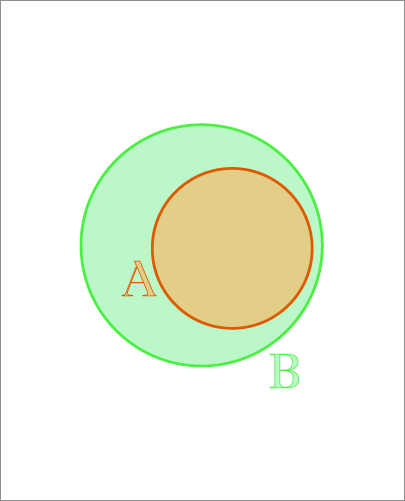
So we have a mental picture of what containment means to us, but there is no way for us to transfer this mental picture directly to the Penrose system and say, "Okay this is what we want when we write isContained(A, B)". Therefore we need to pause for a second, and really think about what it means for a circle to be contained in another circle mathematically.

There are generally 3 scenarios for the containment relationship between 2 circles.

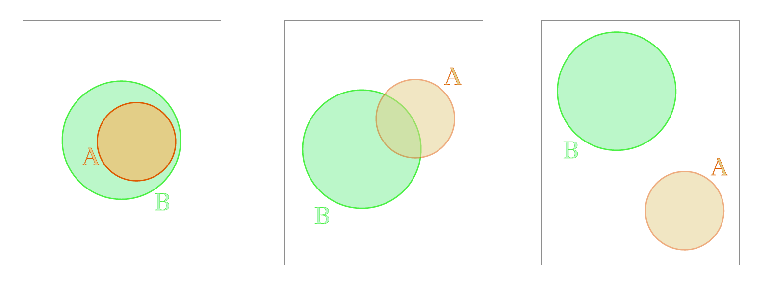
We have completely contained, overlapping but not contained, and completely disjoint. Disjoint means none of the points in circle A is also in circle B, i.e. they do not overlap at all.

The three scenarios are visually obvious to us. We are shown 2 circles, and we can immediately identify their relationship. While Penrose does not have eyes, it speaks math! So, let's try looking at these circles a different way.

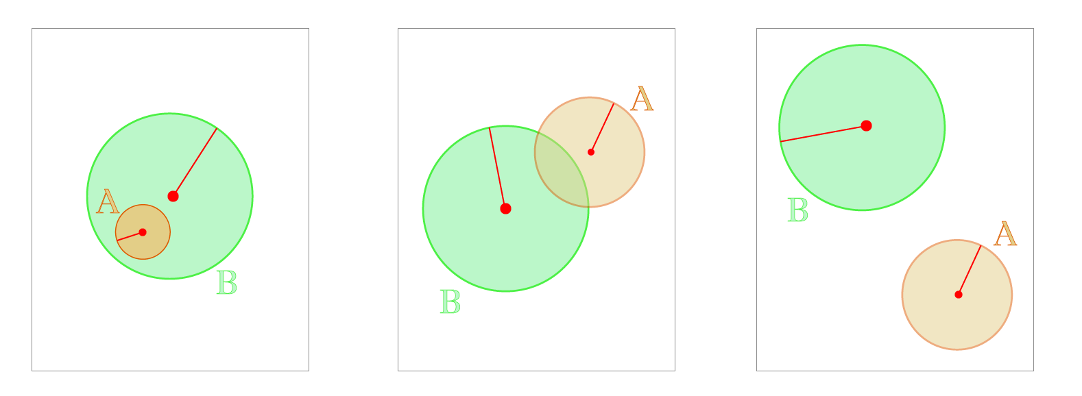
Recall the general equation for a circle where $p$ is some point, $c$ is the center and $r$ is the radius: $||p-c||=r$. This equation is in vector form since Penrose has built-in vector support so we prefer working with them when possible.

The center coordinate and radius are the information we have about any circle, and we will use this information to determine two circle's containment relationship.

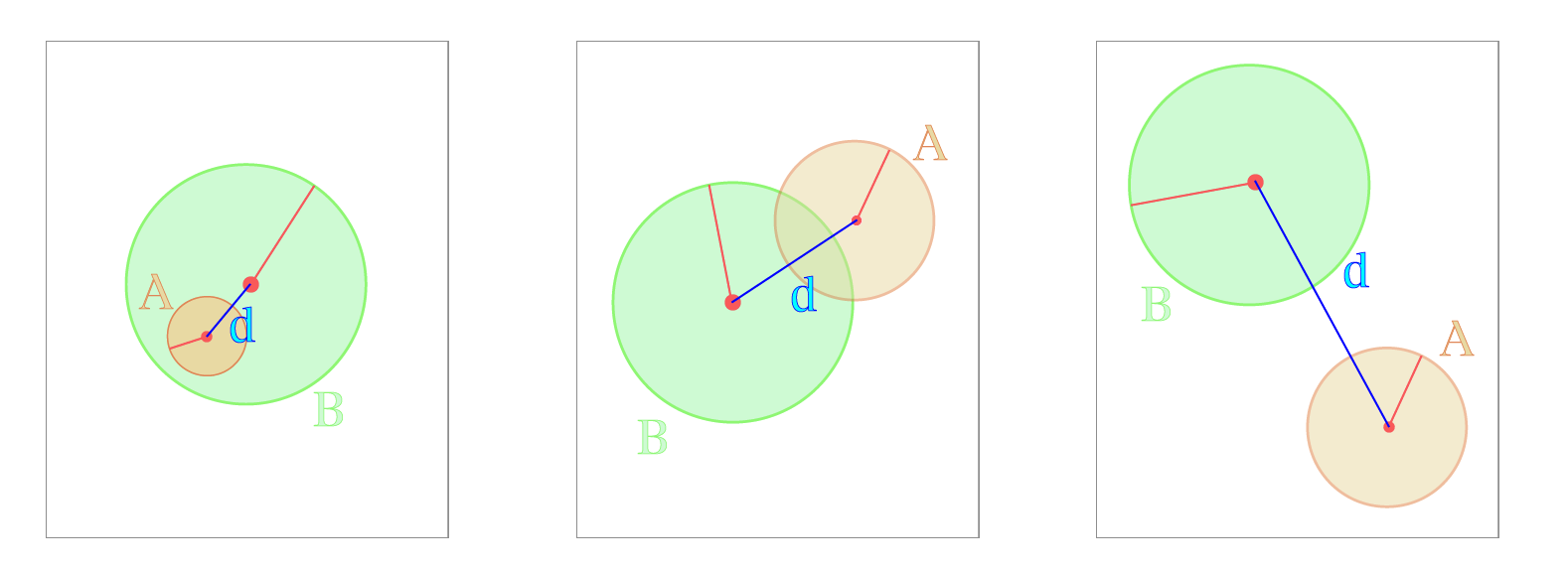
Another piece of information we will be using is the distance $d$ between the radii. Notice how the distance gets progressively bigger as $A$ and $B$ become more disjoint. When $A, B$ are disjoint, we see that $d$'s value is the greatest.

Let's see a scenario when a circle is perfectly contained in another one.

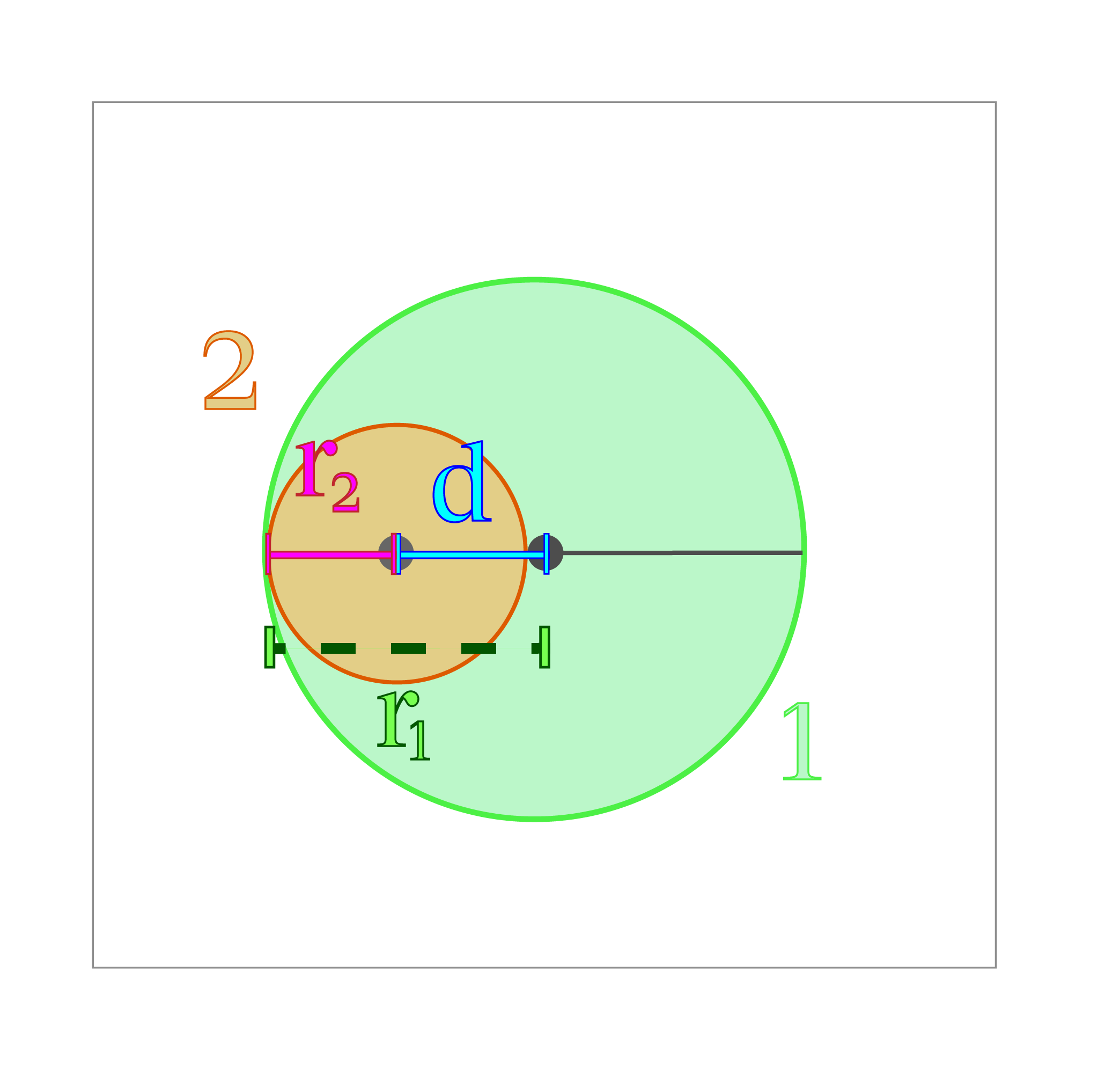
Circle 1 contains circle 2 if and only if circle 1's radius is greater than the distance between their centers, plus circle 2's radius, i.e. $r_1 > d+r_2$. This diagram shows the most illustrative case when Circle 2 is just contained, which we can understand by intuitively reasoning about the directions of change for each degree of freedom:

• If $r_2$ is any smaller, Circle 2 remains contained. If $r_2$ is any larger, clearly Circle 2 is no longer contained.
• If $d$ is any smaller, then Circle 2 remains contained; if $d$ is any larger, then Circle 2 is no longer contained.
• If $r_1$ is any larger, then Circle 2 remains contained; if $r_1$ is any smaller, then Circle 2 is no longer contained.

So, by rearranging the containment expression, we arrive at the energy expression $d - (r_1 - r_2) < 0$.

Here's a short proof. Read on if you are still a bit hesitant. Let $r_{\text{difference}}=r_B-r_A$.

• We know $r_{\text{difference}}<0$ when $r_A > r_B$, i.e. radius of the circle A (that we want to be contained) is greater than the radius of circle B. In that case, A cannot be contained by B. Then we have $d-r_{\text{difference}}>d$.
• We have $r_{\text{difference}} = 0$ when $r_A = r_B$, i.e. the radii of the two circles are equal, and they can be contained in each other if and only if distance $d=r_B=r_A$, then $d-r_{\text{difference}}=d$.
• We have $r_{\text{difference}}>0$ when $r_A < r_B$, i.e. $A$ is a smaller circle than $B$. In that case $A$ is perfectly containable, and $d-r_{\text{difference}} < d$.
• As shown above, we can conclude that as circle $A$ becomes more contained within circle $B$, the value of $d-r_{\text{difference}}$ decreases accordingly.

Concrete: How We Write Constraints

The syntax for writing a constraint works in a way that allows Penrose to use a particular technique called automatic differentiation, autodiff for short. The Penrose system uses autodiff to find the optimized diagram.

1. The Autodiff Code is Built in Typescript

Unlike the tutorials where we were working with file triples in the custom Penrose language, this part of Penrose is fundamentally built in Typescript. As you will see, there are still some key rules and tricks to follow when writing constraints for autodiff. All objectives, constraints, and functions need to be written in a differentiable manner.

2. Autodiff Functions

In order to perform automatic differentiation, Penrose needs to keep track of the operations that are performed on all numbers in an internal graph-based format. As a result, we have to make use of pre-defined Penrose operators and shift away from native Typescript operations such as + and -.

We have unary, binary, trinary, n-ary, and composite operations. The terms unary, binary, etc. refer to the number of objects that are passed into the operation. For example, instead of a + b, we now write add(a, b), which is a binary operator because it takes two inputs, a and b.

The composite operations are accessed through ops.<function-name>. For example, to access the dist operator to find the distance between two points expressed in vector form (say A and B), we'd write ops.dist(A, B).

3. Special Number Types

All numbers are required to be a special type called Num in order to be valid inputs for autodiff functions. Any number is already automatically a Num, and treated as a constant. For example, if we need to do 5 + 3, it's totally fine to just say add(5, 3). Or if one or both of the arguments is a general Num instead of a constant number, that's fine too: for instance, if we have x: Num and y: Num, then add(x, 3), add(5, y), and add(x, y) are all valid.

4. Zero-Based Inequality to Energy Function

For every constraint function we write, we take in shapes and output either a number or a tensor as a penalty. In short, Penrose will try to minimize the outputs of all the constraint functions used for the diagram.

When we write a constraint, for example, we want to constrain one circle s1 to be smaller than another circle s2 by some amount offset. In math, we would require that $r_1 - r_2 > \text{offset}$. An inequality constraint needs to be written in the form $p(x) > 0$ since we penalize the amount the constraint is greater than $0$. So, this constraint is written as $r_1 - r_2 - \text{offset} > 0$, or $p(r_1, r_2) = r_1 - r_2 - \text{offset}$.

Some general rules on writing energy function:

Let's say I want the constraint $f(x) \leq c$ to be true.

1. Translate it to the zero-based inequality $f(x) - c \leq 0$.
2. Translate the inequality constraint into an energy (aka penalty) $E(x) = f(x) - c$, it is greater than $0$ if and only if the constraint is violated. The more the constraint is violated, the higher the energy (i.e. if $f(x)$ is much larger than $c$ then the energy $E(x)$ is also larger than $0$).

5. Negative Outputs of Energy Functions

Previously, we've talked about how we convert everything to zero-based inequality, so what happens when the energy function outputs a negative value? It simply means that the constraint is satisfied.

6. Accessing a Value of a Shape's Field

One common operation is to access the parameter of a shape via shapeName.propertyName.contents, which will return a Num. For example, if you have a circle c as input, and you want its radius, c.r.contents will give you something like 5.0 (of type Num).

Objectives Example: Circle Repel

Unlike constraints, which are binary in that they are either satisfied ($\leq 0$) or unsatisfied ($> 0$), objective functions should output the "badness" of the inputs (as a number or Tensor), and have local minima where we want the solution to be.

Now we look at an objective that makes two circles repel, encouraging the two circles to stay far away from each other.

const repel = (s1: Circle<Num>, s2: Circle<Num>, weight: Num = 10e6) => {
  const epsDenom = 10e-6;
  const res = inverse(
    add(ops.vdistsq(s1.center.contents, s2.center.contents), epsDenom),
  );
  return mul(res, weight);
};

Let's look at this code together step by step:

• Input: The function takes inputs similar to the constraint functions we just looked at. We add a parameter, weight, which is present because repel() typically needs to have a weight multiplier since its magnitude is small.
• Operations: Here we use 3 autodiff functions:
  • inverse, which returns 1 / v
  • mul performs multiplication
  • ops.vdistsq returns the squared Euclidean distance between vectors v and w. Remember we useops to access composite functions that work on vectors.
• Logic: We will convert the math done in the second line of the function to its corresponding mathematical equation.

$\frac{1}{||C_A - C_B||^2 } = \frac{1}{d^2}$

So essentially, the repel function takes in two circles and returns the inverse of the distance between them squared, i.e. we plug in the distance $d$ between the circles as an input to the $f(x)=\frac{1}{x^2}$ function.

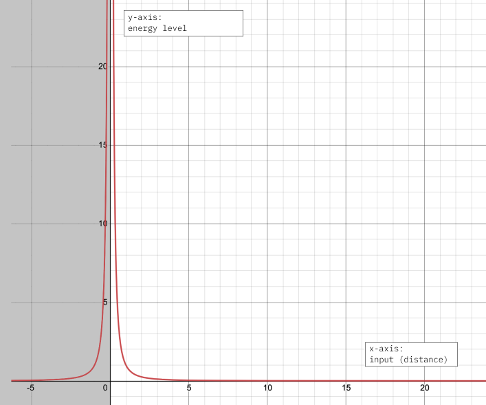
If you look at the graph of $f(x)=\frac{1}{x^2}$, notice how the output increases as $d$ decreases, i.e. the higher penalty value we return. We block the negative horizontal range since we cannot have negative distances.

We then return the value above multiplied by the weight, and let's take a look at the graph of $\frac{10e6}{x^2}$.

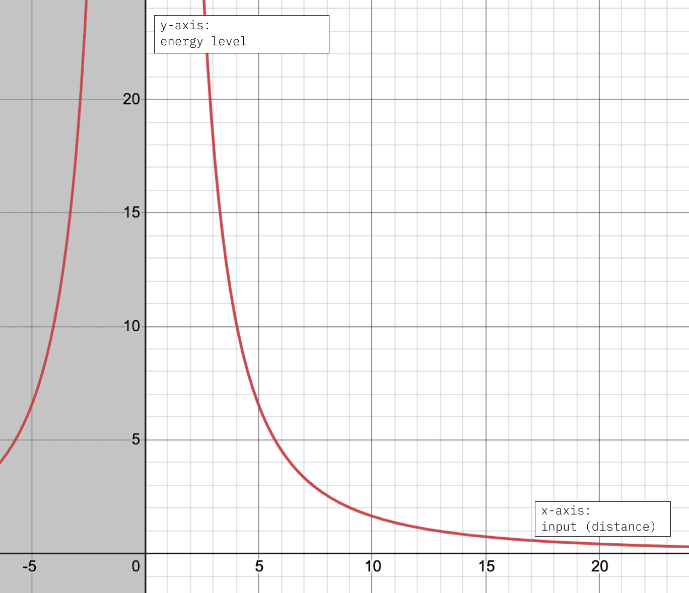
If you compare the two graphs above, you can see how we expanded the range of extreme high outputs by multiplying $\frac{1}{x^2}$ with a big constant.

Exercises

• Write a constraint that makes 2 circles disjoint from each other. Remember disjoint means that the two circles do not overlap at all.
• Write a new disjoint function that allows padding, i.e. the minimum distance between two circles will be the padding value.

Exercise Solutions

/* d(c1, c2) + r1 + r2 >= 0 */
const disjoint = (s1: Circle<Num>, s2: Circle<Num>) => {
  const res = add(s1.r.contents, s2.r.contents);
  return sub(res, ops.vdist(s1.center.contents, s2.center.contents));
};

/* d(c1, c2) + r1 + r2 >= padding */
const disjointPadding = (s1: Circle<Num>, s2: Circle<Num>, padding: Num) => {
  const res = add(add(s1.r.contents, s2.r.contents), padding);
  return sub(res, ops.vdist(s1.center.contents, s2.center.contents));
};

Takeaways

In this tutorial, we took a leap from being users of the Penrose system to being developers contributing to the Penrose system. In particular, we learned the following things:

• Diagramming can be encoded as an optimization problem, and Penrose uses numerical operations.
• Constraints and objectives are implemented as energy functions, and the outputs of an energy function is called energy.
• The lower the energy, the better! A diagram with low energy for all of its constraints and objectives is a good diagram.
• To write an energy function, we use autodiff functions with special number types.